Fast Fourier Transform (FFT) simple usage

How to build spectrum of signal? Here is simple, but detailed example of Matlab's fft() function usage. Also I showed how correctly plot discrete time signal and discrete spectrum of signal.

1. Clear command window, memory and close all plot windows, that were opened before.

clc;
clear all;
close all;

2. Set sample frequency. According to Kotel'nikov's theorem sample frequency mast be two or more times larger than the biggest spectral component in signal. Let's take sampling frequency of 1000 Hz.

Fs = 1000; % sampling frequency

then the spectrum of our signal will reach up to 500 Hz.

3. Calculate the sampling period (in seconds).

dT = 1/Fs; % sampling period

4. Determine the number of samples in the signal:

N = 4096; % number of signal samples

5. We define the vector of time:

t = (1:N)*dT; % vector of time

6. Form a digital signal. For simplicity, we take a sinusoidal signal with a frequency of 10 Hz.

u = sin(2*pi*10*t); % discrete signal

7. Initialize the window to display the plot. We define the ability to display multiple graphs in one window. Enable the grid.

figure; % initialize the window to display the plot
hold on; % ability to display multiple graphs in one window
grid on; % enable the grid

8. We derive the signal as a function of time:

plot(t(1:N/2),u(1:N/2)); % construct a given signal as a function of time

9. Accents marks:

xlabel('t, sec');
ylabel('u, volts');
title('Input signal');

Window with the signal plot

10. We find the spectrum of the signal using FFT (Fast Fourier Transform) use built-in Matlab function fft.

U = fft(u);

11. We define the vector of frequency:

f = (0:N/2-1)*(Fs/N);

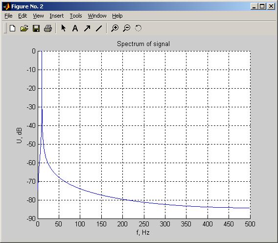
12. Building the spectrum

figure;
hold on;
grid on;
plot(f,20*log10(abs(U(1:N/2))/max(abs(U(1:N/2)))));
xlabel('f, Hz');
ylabel('U, dB');
title('Spectrum of signal');

Window with the spectrum of the signal